探索ggml的实现
本文主要介绍ggml的调试入门环境搭建、ggml的核心数据结构、内存管理与布局、计算图构建与执行、以及gguf文件格式构成,会分成多个小节介绍。
本文起源于作者ggml学习过程中了解的资料,包括xsxszab的ggml-deep-dive系列文章 、以及阅读源码,记录和分享自己的理解过程。(感谢xsxszab绘制的关于内存布局的图例,为ggml的理解更加浅显易懂。)
ggml是采用c/c++编写高度优化的tensor张量计算库,没有外部依赖。存在不同的backend实现,从mac的metal、x86的avx实现以及arm的neon指令实现、gpu的cuda、hip、opencl等实现。llama.cpp项目就是使用ggml进行模型加载、推理的。
探索ggml的实现–vscode调试环境的搭建
在阅读源码的时候,找一个最简单的example例子跑通,然后跟着源码进行调试,是很快理解原理的一种方法。
在linux、或者mac下都方便编译。
编译依赖:
gcc/g++或者 clang编译
cmake: 用于管理构建项目
ccache:可选项,加快编译速度用
Bash clone https://github.com/ggml-org/ggml.git
上面的依赖安装很简单,以ubuntu为例:
Bash update
install -y gcc g++ cmake ccache
配置调试目标
ggml的example中包括了很多例子,先从简单的例子看起。
Bash
修改项目的cmake配置,即添加-g方便debug调试。找到examples/simple/CMakeLists.txt配置文件,为simple-ctx这个可执行文件添加-g参数。
Bash ( TEST_TARGET simple-ctx)
( ${ TEST_TARGET } simple-ctx.cpp)
( ${ TEST_TARGET } PRIVATE -g)
( ${ TEST_TARGET } PRIVATE ggml)
Bash -B build -S . -DCMAKE_BUILD_TYPE= DEBUG
--build build
Bash build/src/libggml.so
ELF 64 -bit LSB shared object, x86-64, version 1 ( SYSV) , dynamically linked, BuildID[ sha1]= db376e303daeef672c8002ed6cebed1da303a706, with debug_info, not stripped
vscode配置debug
点击右边的Run and Debug按钮,create a launch.json file,创建一个配置文件,把下面的内容粘贴进去。
JSON {
"version" : "0.2.0" ,
"configurations" : [
{
"name" : "debug simple-ctx" ,
"type" : "lldb" ,
"request" : "launch" ,
"program" : "${workspaceFolder}/build/bin/simple-ctx" ,
"cwd" : "${workspaceFolder}"
}
]
}
可以看到,通过上面的编译debug模式和添加-g参数,可以进入可执行程序和ggml.so库的源码进行调试了了。
探索ggml的实现–张量表示
ggml_tensor 数据结构
在GGML中通过ggml_tensor结构体表示张量,结构体定义如下:
C++ // n-dimensional tensor
struct ggml_tensor {
// 张量的数据类型:例如GGML_TYPE_F32,GGML_TYPE_F16,GGML_TYPE_Q4_0
enum ggml_type type ;
struct ggml_backend_buffer * buffer ;
// 最大维度为4,GGML_MAX_DIMS为4
// ne存储张量每个维度的元素个数
// nb存储张量每个维的元素大小
int64_t ne [ GGML_MAX_DIMS ]; // number of elements
size_t nb [ GGML_MAX_DIMS ]; // stride in bytes:
// nb[0] = ggml_type_size(type)
// nb[1] = nb[0] * (ne[0] / ggml_blck_size(type)) + padding
// nb[i] = nb[i-1] * ne[i-1]
// 张量op类型,在计算图中作为op node,后面会提到
// 例如矩阵乘类型,GGML_OP_MUL_MAT
// compute data
enum ggml_op op ;
// op params - allocated as int32_t for alignment
int32_t op_params [ GGML_MAX_OP_PARAMS / sizeof ( int32_t )];
int32_t flags ;
// 指针指向此张量的src张量
// 例如矩阵乘op tensor的src张量是矩阵A tensor和矩阵B tensor
struct ggml_tensor * src [ GGML_MAX_SRC ];
// 描述张量视图,如果此张量是另一个张量(base张量)的视图,则指向base张量
// source tensor and offset for views
struct ggml_tensor * view_src ;
// 视图张量的偏移量
size_t view_offs ;
// 存储张量的数据
void * data ;
// 张量的名称
char name [ GGML_MAX_NAME ];
void * extra ; // extra things e.g. for ggml-cuda.cu
char padding [ 8 ];
};
通过一个例子学习tensor
在examples文件夹中添加一个simple-add.cpp的文件,添加如下内容:
C++ #include "ggml.h"
#include "ggml-cpu.h"
#include <cstring>
#include <iostream>
#include <vector>
int main () {
struct ggml_init_params params {
/*.mem_size =*/ 1024 * 1024 * 1024 + ggml_graph_overhead (),
/*.mem_buffer =*/ NULL ,
/*.no_alloc =*/ false ,
};
ggml_context * ctx = ggml_init ( params );
// --------------------
// Modify this section to test different tensor computations
float a_data [ 3 * 2 ] = {
1 , 2 ,
3 , 4 ,
5 , 6
};
float b_data [ 3 * 2 ] = {
1 , 1 ,
1 , 1 ,
1 , 1
};
// 因为ggml中tensor表示和pytorch相反,因此3行2列的矩阵,表示为[2, 3]
ggml_tensor * a = ggml_new_tensor_2d ( ctx , GGML_TYPE_F32 , 2 , 3 );
ggml_tensor * b = ggml_new_tensor_2d ( ctx , GGML_TYPE_F32 , 2 , 3 );
memcpy ( a -> data , a_data , ggml_nbytes ( a ));
memcpy ( b -> data , b_data , ggml_nbytes ( b ));
ggml_tensor * result = ggml_add ( ctx , a , b );
// --------------------
struct ggml_cgraph * gf = ggml_new_graph ( ctx );
ggml_build_forward_expand ( gf , result );
ggml_graph_compute_with_ctx ( ctx , gf , 1 );
std :: vector < float > out_data ( ggml_nelements ( result ));
memcpy ( out_data . data (), result -> data , ggml_nbytes ( result ));
ggml_free ( ctx );
return 0 ;
}
CMake #
# simple-add
set ( TEST_TARGET simple-add )
add_executable ( ${ TEST_TARGET } simple-add.cpp )
target_compile_options ( ${ TEST_TARGET } PRIVATE -g )
target_link_libraries ( ${ TEST_TARGET } PRIVATE ggml )
Bash p *a
( ggml_tensor) {
type = GGML_TYPE_F32
buffer = nullptr
ne = ([ 0 ] = 2 , [ 1 ] = 3 , [ 2 ] = 1 , [ 3 ] = 1 )
nb = ([ 0 ] = 4 , [ 1 ] = 8 , [ 2 ] = 24 , [ 3 ] = 24 )
op = GGML_OP_NONE
op_params = {
[ 0 ] = 0
[ 1 ] = 0
[ 2 ] = 0
[ 3 ] = 0
[ 4 ] = 0
[ 5 ] = 0
[ 6 ] = 0
[ 7 ] = 0
[ 8 ] = 0
[ 9 ] = 0
[ 10 ] = 0
[ 11 ] = 0
[ 12 ] = 0
[ 13 ] = 0
[ 14 ] = 0
[ 15 ] = 0
}
flags = 0
src = {
[ 0 ] = nullptr
[ 1 ] = nullptr
[ 2 ] = nullptr
[ 3 ] = nullptr
[ 4 ] = nullptr
[ 5 ] = nullptr
[ 6 ] = nullptr
[ 7 ] = nullptr
[ 8 ] = nullptr
[ 9 ] = nullptr
}
view_src = nullptr
view_offs = 0
data = 0x00007fffb75eb1b0
name = ""
extra = 0x0000000000000000
padding = ""
}
tensor的内存布局
f32矩阵
对于ne的理解,比如一个RGB的图片,width为1920,height为1080, 用pytorch表示维度信息就是[1, 3, 1080, 1920],即[N, C, H, W]。而在GGML中,这个维度信息表示为:
[1920, 1080, 3, 1]。
C++ type = GGML_TYPE_F32
buffer = nullptr
ne = ([ 0 ] = 2 , [ 1 ] = 3 , [ 2 ] = 1 , [ 3 ] = 1 )
// 4表示第一维每个元素所占字节数。8表示每行元素间隔8个字节,也就是间隔两个元素。
// 也就是在内存存储的布局是row major连续存储的
nb = ([ 0 ] = 4 , [ 1 ] = 8 , [ 2 ] = 24 , [ 3 ] = 24 )
op = GGML_OP_NONE
量化矩阵
在上面的例子任意地方加一行表示一个量化矩阵。
C++ ggml_tensor * c = ggml_new_tensor_2d ( ctx , GGML_TYPE_Q4_0 , 32 , 6 );
通过p *c 可以查看矩阵的详细信息。
Bash p *c
( ggml_tensor) {
type = GGML_TYPE_Q4_0
buffer = nullptr
ne = ([ 0 ] = 32 , [ 1 ] = 6 , [ 2 ] = 1 , [ 3 ] = 1 )
nb = ([ 0 ] = 18 , [ 1 ] = 18 , [ 2 ] = 108 , [ 3 ] = 108 )
op = GGML_OP_NONE
......
}
C++ typedef uint16_t ggml_half ;
#define QK4_0 32
typedef struct {
// 16bit存储delta信息, 2个字节
ggml_half d ; // delta
// 8bit数组,数组长度为:16, 16个字节
uint8_t qs [ QK4_0 / 2 ]; // nibbles / quants
} block_q4_0 ;
static_assert ( sizeof ( block_q4_0 ) == sizeof ( ggml_half ) + QK4_0 / 2 , "wrong q4_0 block size/padding" );
我们ne[0]和ne[1]分别为32, 16,表示了32行和16列的int4矩阵。而nb[0]为18,表示GGML的q4_0量化将32个int4元素组合在一起,再加上一个16位的差值,每组共18字节。
[32, 6, 1, 1]的Q4_0数组就可以看成[1,6,1,1],因为32个元素为内存上的最小寻址单元。更高维度的情况下,nb[i] = nb[i-1] * ne[i]。
矩阵permute重排列
看一个pytorch例子,了解permute是什么?permute就是对数据的维度变化顺序
C++ import torch
import numpy as np
a = np . array ([[[ 1 , 2 , 3 ],[ 4 , 5 , 6 ]]])
unpermuted = torch . tensor ( a )
print ( unpermuted . size ()) # —— > torch . Size ([ 1 , 2 , 3 ])
permuted = unpermuted . permute ( 2 , 0 , 1 )
print ( permuted . size ()) # —— > torch . Size ([ 3 , 1 , 2 ])
C++ tensor ([[[ 1 , 4 ]],
[[ 2 , 5 ]],
[[ 3 , 6 ]]]) # print ( permuted )
再看ggml中的permute操作,添加如下例子:
C++ ggml_tensor * before = a ;
// Same as PyTorch's permute()
ggml_tensor * after = ggml_permute ( ctx , before , 1 , 0 , 2 , 3 );
Bash p *before
( ggml_tensor) {
type = GGML_TYPE_F32
buffer = nullptr
ne = ([ 0 ] = 2 , [ 1 ] = 3 , [ 2 ] = 1 , [ 3 ] = 1 )
nb = ([ 0 ] = 4 , [ 1 ] = 8 , [ 2 ] = 24 , [ 3 ] = 24 )
op = GGML_OP_NONE
view_src = nullptr
view_offs = 0
data = 0x00007fffb77eb1b0
}
p *after
( ggml_tensor) {
type = GGML_TYPE_F32
buffer = nullptr
ne = ([ 0 ] = 3 , [ 1 ] = 2 , [ 2 ] = 1 , [ 3 ] = 1 )
nb = ([ 0 ] = 8 , [ 1 ] = 4 , [ 2 ] = 24 , [ 3 ] = 24 )
op = GGML_OP_PERMUTE
view_src = 0x00007fffb77eb060
view_offs = 0
data = 0x00007fffb77eb1b0
name = " (permuted)"
}
C++ // Pseudo-code representation of tensor's memory layout
data = [ 1 , 2 , 3 , 4 , 5 , 6 ]
// Accessing row 1 before permutation, nb[0] = 4
// 1, 2,
// 3, 4,
// 5, 6
e0 = ( p + nb [ 0 ] * 0 ) = 1
e1 = ( p + nb [ 0 ] * 1 ) = 2
// Accessing row 1 after permutation, nb[0] = 8
// [[1,3,5],
// [2,4,6]]
e0 = ( p + nb [ 0 ] * 0 ) = 0
e1 = ( p + nb [ 0 ] * 1 ) = ( p + 8 ) = 3
e1 = ( p + nb [ 0 ] * 2 ) = ( p + 16 ) = 5
张量视图
视图可以对张量内存进行复用,避免拷贝、避免低效的为每个张量分配一个独特的内存块。
以ggml_cpy操作为例,拷贝的b tensor就是相对于a创建的一个视图。
C++ // ggml_cpy
static struct ggml_tensor * ggml_cpy_impl (
struct ggml_context * ctx ,
struct ggml_tensor * a ,
struct ggml_tensor * b ) {
GGML_ASSERT ( ggml_nelements ( a ) == ggml_nelements ( b ));
// make a view of the destination
struct ggml_tensor * result = ggml_view_tensor ( ctx , b );
if ( strlen ( b -> name ) > 0 ) {
ggml_format_name ( result , "%s (copy of %s)" , b -> name , a -> name );
} else {
ggml_format_name ( result , "%s (copy)" , a -> name );
}
result -> op = GGML_OP_CPY ;
result -> src [ 0 ] = a ;
result -> src [ 1 ] = b ;
return result ;
}
以LLM中Q、K、V tensor为例,下面的Qcur、Kcur、Vcur可以表示成创建的tensor_input的一部分。所以视图不用是base tensor的全部,可以只是一部分,通过offset可以设置相对base tensor的偏移量。
C++ struct ggml_tensor * tensor_input = ggml_new_tensor_2d ( ctx , GGML_TYPE_32 , 768 * 3 , seq_len );
// Create a view tensor of shape (768, seq_len) with offset 0
// The last parameter of ggml_view_2d specifies the view's offset (in bytes)
struct ggml_tensor * Qcur = ggml_view_2d ( ctx0 , tensor_input , 768 , seq_len , cur -> nb [ 1 ], 0 * sizeof ( float ) * 768 );
// Create a view tensor of shape (768, seq_len) with offset 768
struct ggml_tensor * Kcur = ggml_view_2d ( ctx0 , tensor_input , 768 , seq_len , cur -> nb [ 1 ], 1 * sizeof ( float ) * 768 );
// Create a view tensor of shape (768, seq_len) with offset 768 * 2
struct ggml_tensor * Vcur = ggml_view_2d ( ctx0 , tensor_input , 768 , seq_len , cur -> nb [ 1 ], 2 * sizeof ( float ) * 768 );
探索ggml的实现–GGML的内存管理
本小节通过最简单的一个例子, ./examples/simple/simple-ctx.cpp,理解GGML实现两个矩阵执行矩阵乘法的核心工作流程。
这个例子具有以下特点,也因此作为我们理解的起点。
!!![warning]
GGML采用c语言风格实现,所以在内存管理上,通过struct中的指针和偏移量来管理内存,我们需要跟踪指针值、计算偏移量,来理解它的内存布局。
认识ggml_context
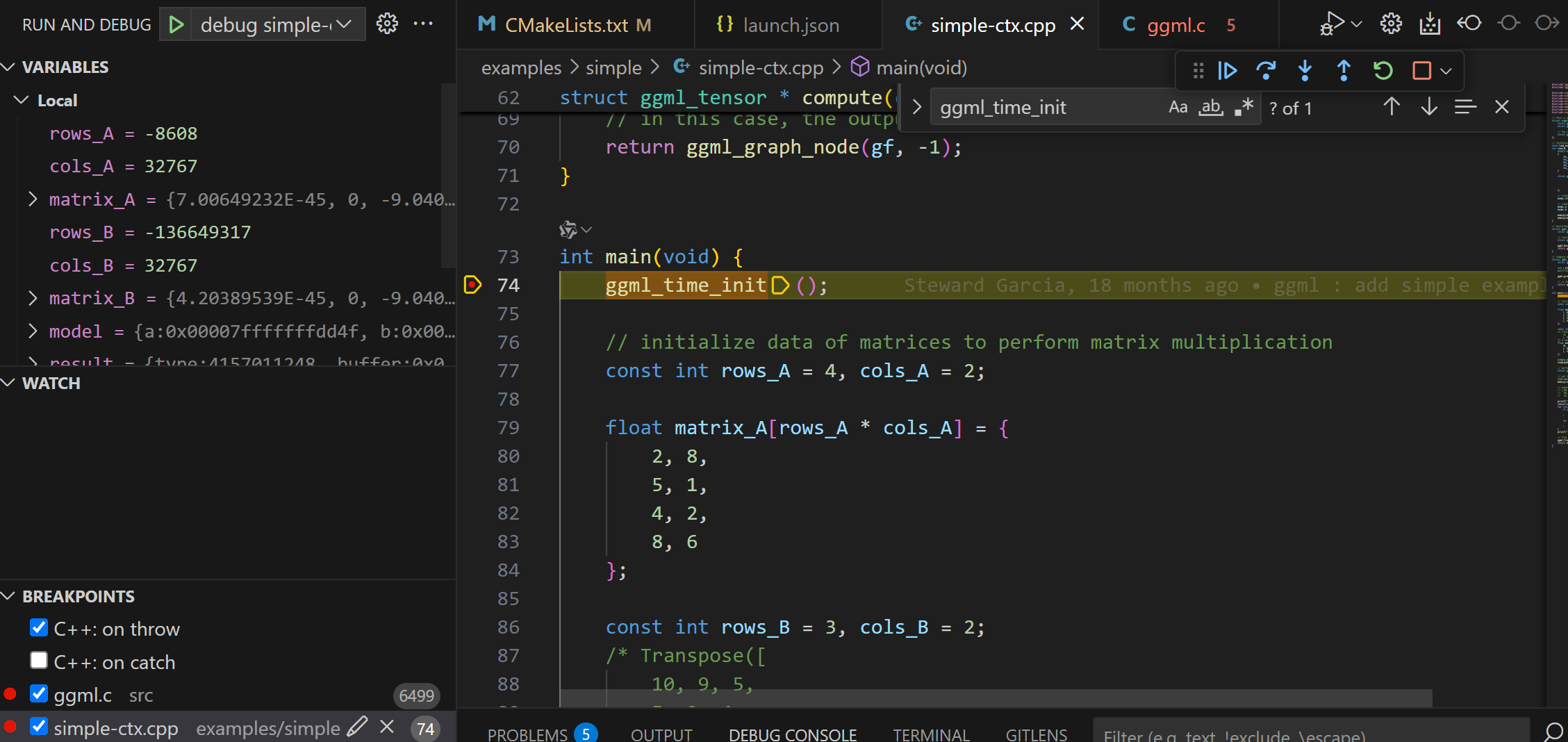
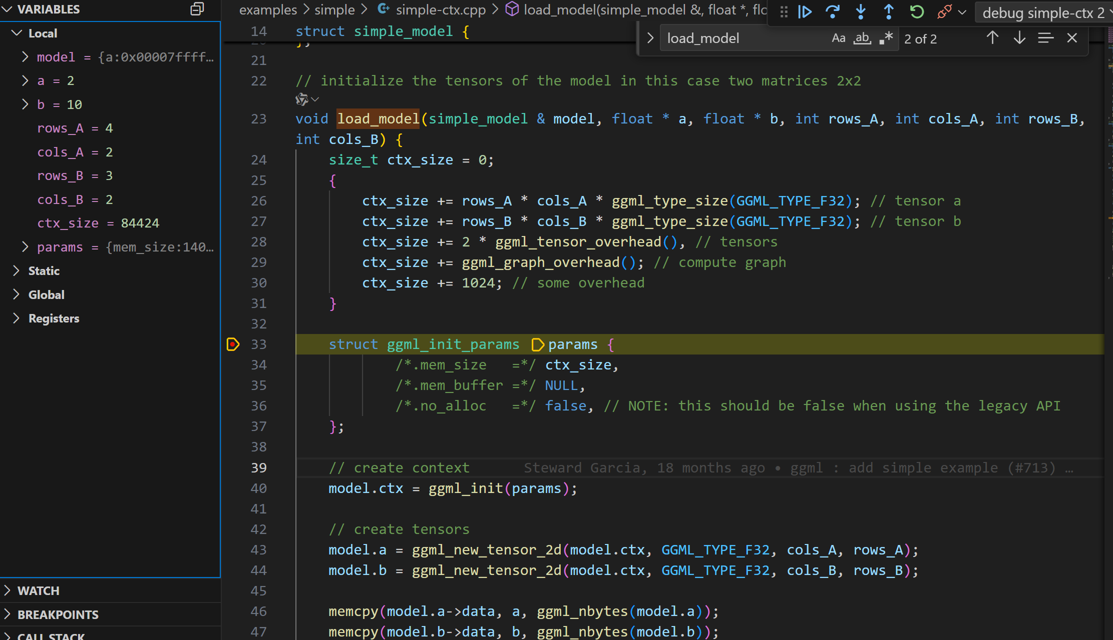
跳过不重要的函数(比如: ggml_time_init),断点debug进入load_model函数。首先看到一个ctx_size的计算,通过ctx_size作为参数,调用了ggml_init函数, 初始化了struct ggml_context *。
暂时先跳过复杂的ctx_size计算,重点关注这个GGML最重要的函数之一:ggml_init。
理解ggml_init
ggml_init函数接受一个参数ggml_init_params,这个参数中包含内存分配的参数。
mem_size_: 内存池大小,也就是ctx_size(提前计算出来的)
mem_buffer_: 内存池,也就是ctx_buffer,这个内存池用于存储ggml_tensor结构体和数据。这里传递的NULL初始化,表示由内部分配
no_alloc_: 是否使用用户传递的内存池,如果为true,则使用用户传递的内存池。这个传递的false,表示由内部分配内存池。
C++ struct ggml_context * ggml_init ( struct ggml_init_params params ) {
// ......
}
struct ggml_init_params {
// memory pool
size_t mem_size ; // bytes
void * mem_buffer ; // if NULL, memory will be allocated internally
bool no_alloc ; // don't allocate memory for the tensor data
};
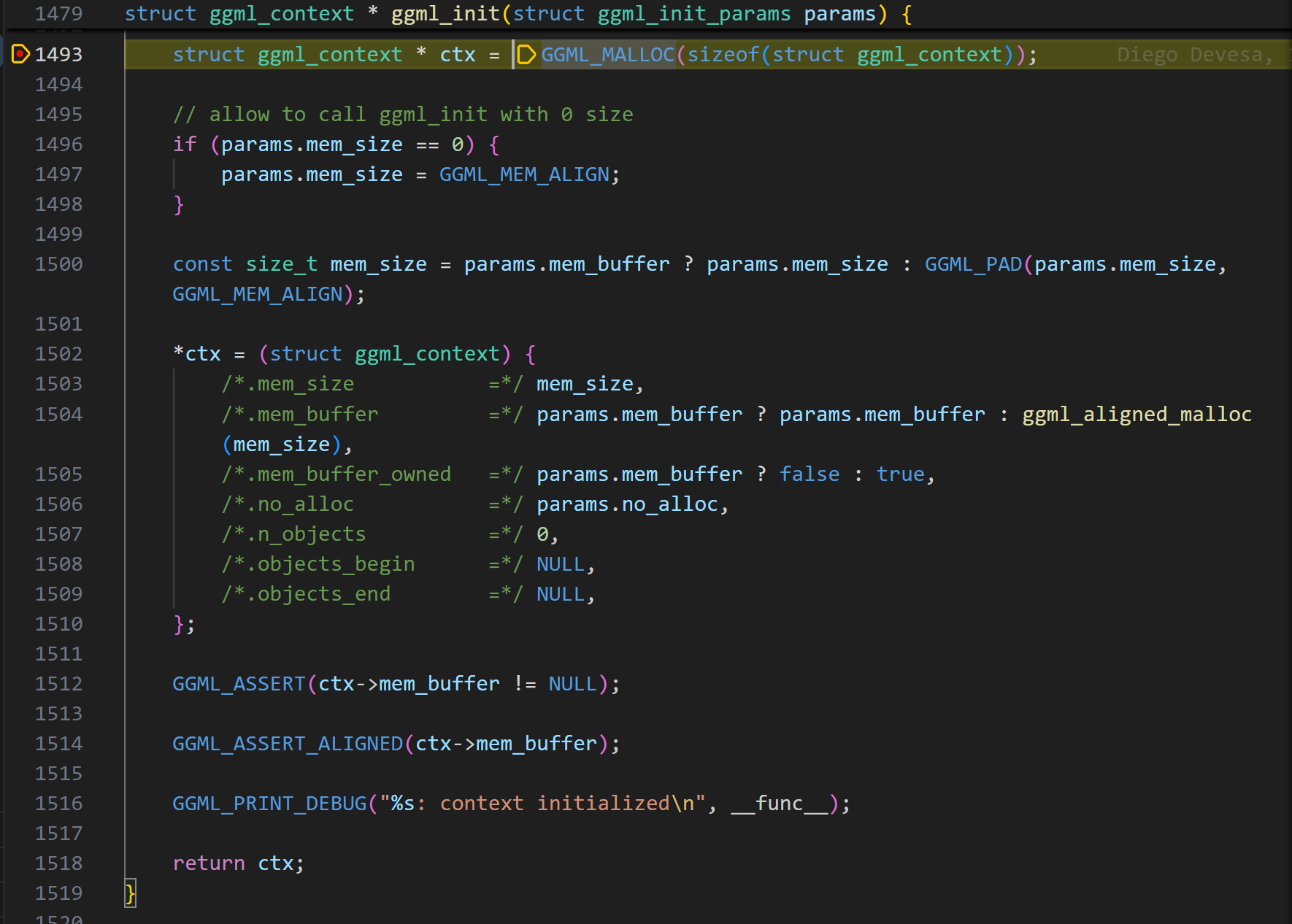
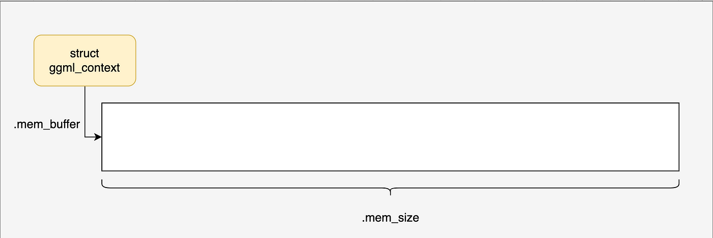
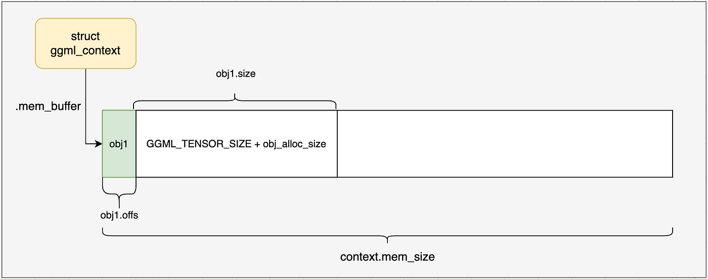
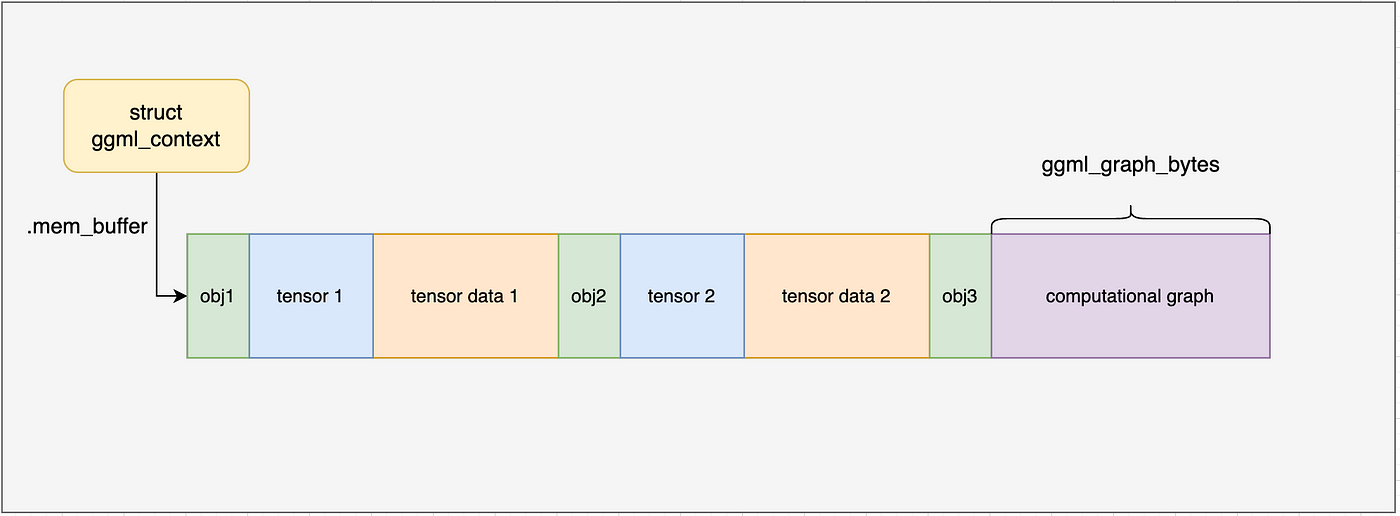
进入ggml_init函数,可以看到,首先在堆上分配了一个struct ggml_context *。
到这里,ggml_context内存布局如下图所示,我们接下来会一步一步了解内部的进一步分配。
GGML的tensor表示
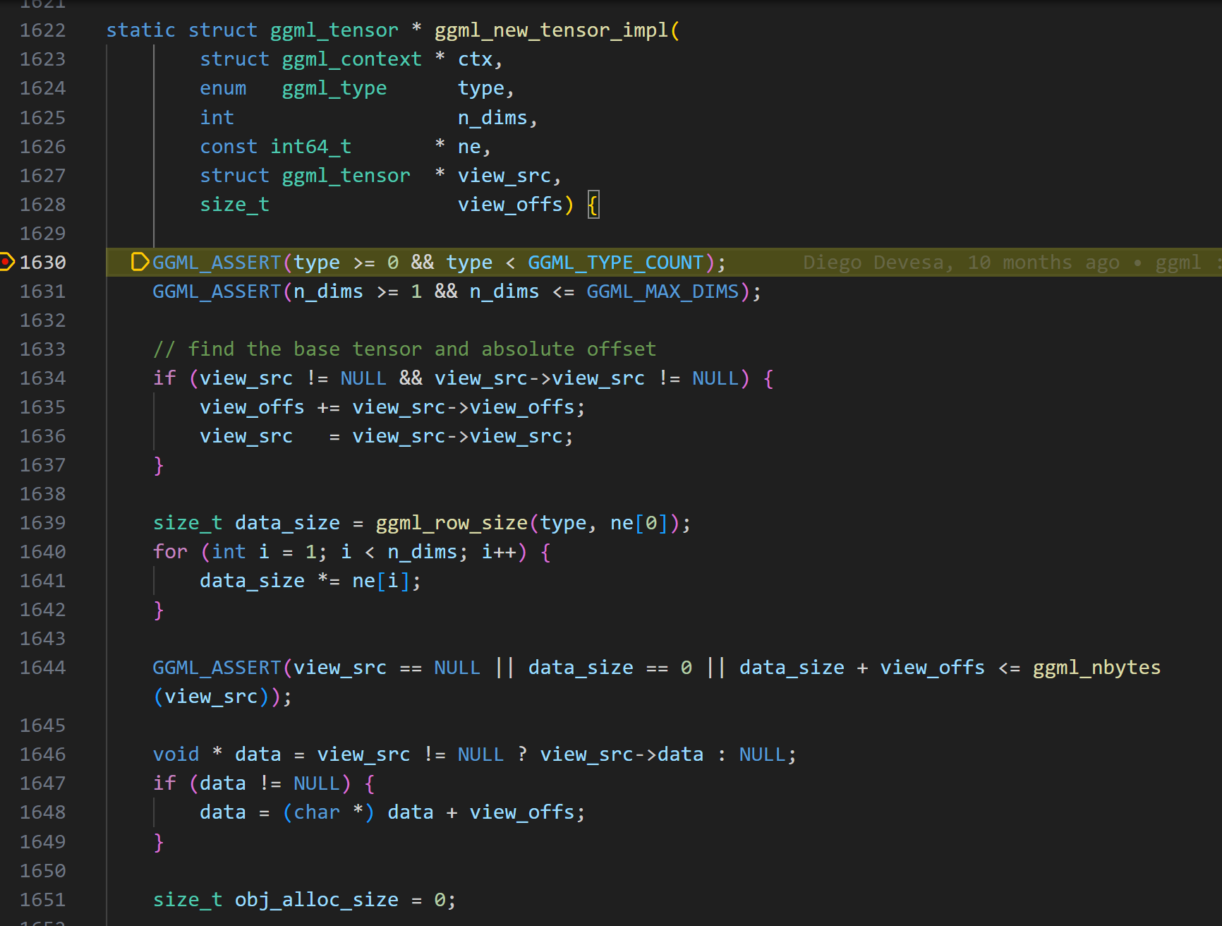
在ggml_init函数执行完成后,紧接着就是对两个矩阵tensor的创建和内存赋值。包括了ggml_new_tensor_2d的调用,一直调用到真正的实现函数ggml_new_tensor_impl。
C++ // create tensors
model . a = ggml_new_tensor_2d ( model . ctx , GGML_TYPE_F32 , cols_A , rows_A );
model . b = ggml_new_tensor_2d ( model . ctx , GGML_TYPE_F32 , cols_B , rows_B );
memcpy ( model . a -> data , a , ggml_nbytes ( model . a ));
memcpy ( model . b -> data , b , ggml_nbytes ( model . b ));
关于view_src的内容可以跳过,主要用于处理张量视图,现在可以不用关心。
首先,一个问题就是:GGML的张量维度是如何表示的?
这里我们可以和pytorch的张量表示进行对比,因为你可以发现,它们的表示方式正好相反。
ggml采用一个四维数组表示shape信息。在pytorch中一个[batch, channels, height, width]的张量,ggml中表示为[width, height, channels, batch]。
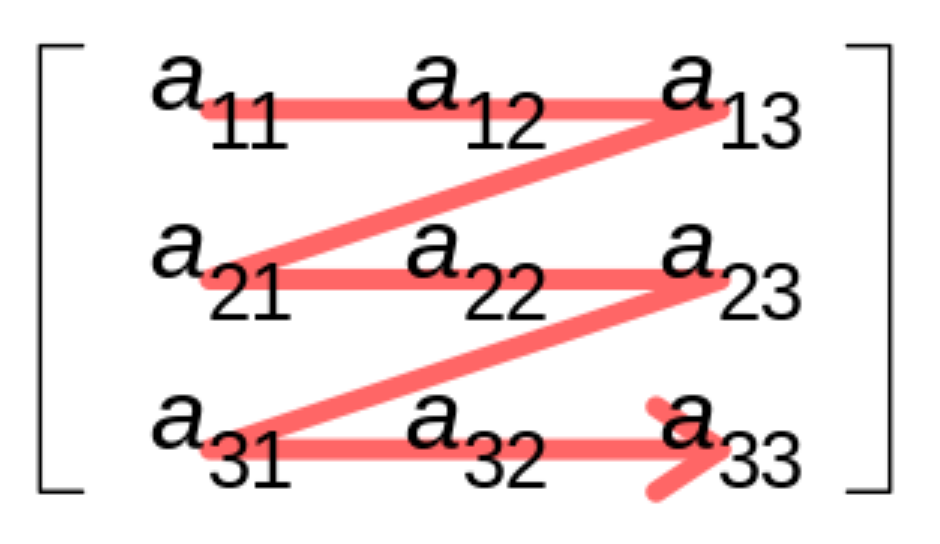
pytorch从最外层到最内层的数据,是从左到右表示的。这里最内层,表示在内存存储上连续的维度。
比如row优先存储,一个3 * 4的矩阵(3行,4列),那最内层维度就是列,也就是4列。pytorch表示为[3, 4],ggml表示为[4, 3]。
上面计算出的data_size,先计算单行的size,然后乘以行数,得到矩阵的size。这里的type是float32类型,如果是量化类型,size就会不同,后面用到在讨论。
C++ size_t obj_alloc_size = 0 ;
if ( view_src == NULL && ! ctx -> no_alloc ) {
// allocate tensor data in the context's memory pool
obj_alloc_size = data_size ;
}
struct ggml_object * const obj_new = ggml_new_object ( ctx , GGML_OBJECT_TYPE_TENSOR , GGML_TENSOR_SIZE + obj_alloc_size );
GGML_ASSERT ( obj_new );
如果view_src为空,且no_alloc为false,则调用ggml_new_object函数,分配一个struct ggml_object *,并初始化。分配的size就是tensor的size,这里就是data_size。
!!! [warning]
view_src表示该obj是其它内存的视图,不需要分配内存,直接复用内存。
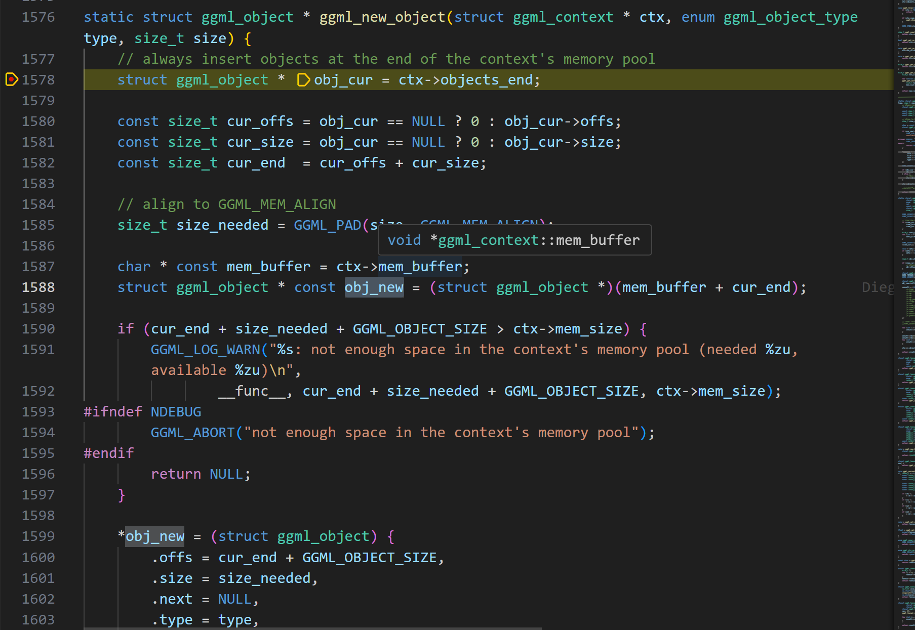
分配的ggml_object结构体有什么用呢?
理解ggml_new_object
直接看代码,可能有点困难,我们对关键点进行总结。
在这个例子中,我们首先计算了context的size,据此分配了ggml_context。接下来的内存分配,包括obj的分配,都是在context的memory pool中完成。
ggml_object的定义可以看出,有一个next指针指向下一个ggml_object。因此它是通过链表来管理内存的,每个ggml_object对象都是一个链表节点。
初始状态下,ggml_object的objects_begin和objects_end都为NULL,表示这个链表为空。
ggml_object的用途是什么呢?ggml通过它来隐式的管理各种资源–包括tensor张量、计算图、work buffer等。链接具有O(n)的查找时间复杂度。
分配一个ggml_object对象,需要多大的内存呢?
C++ struct ggml_object * const obj_new = ggml_new_object ( ctx , GGML_OBJECT_TYPE_TENSOR , GGML_TENSOR_SIZE + obj_alloc_size );
static const size_t GGML_TENSOR_SIZE = sizeof ( struct ggml_tensor );
以这里ggml_object分配的是tensor类型为例子:
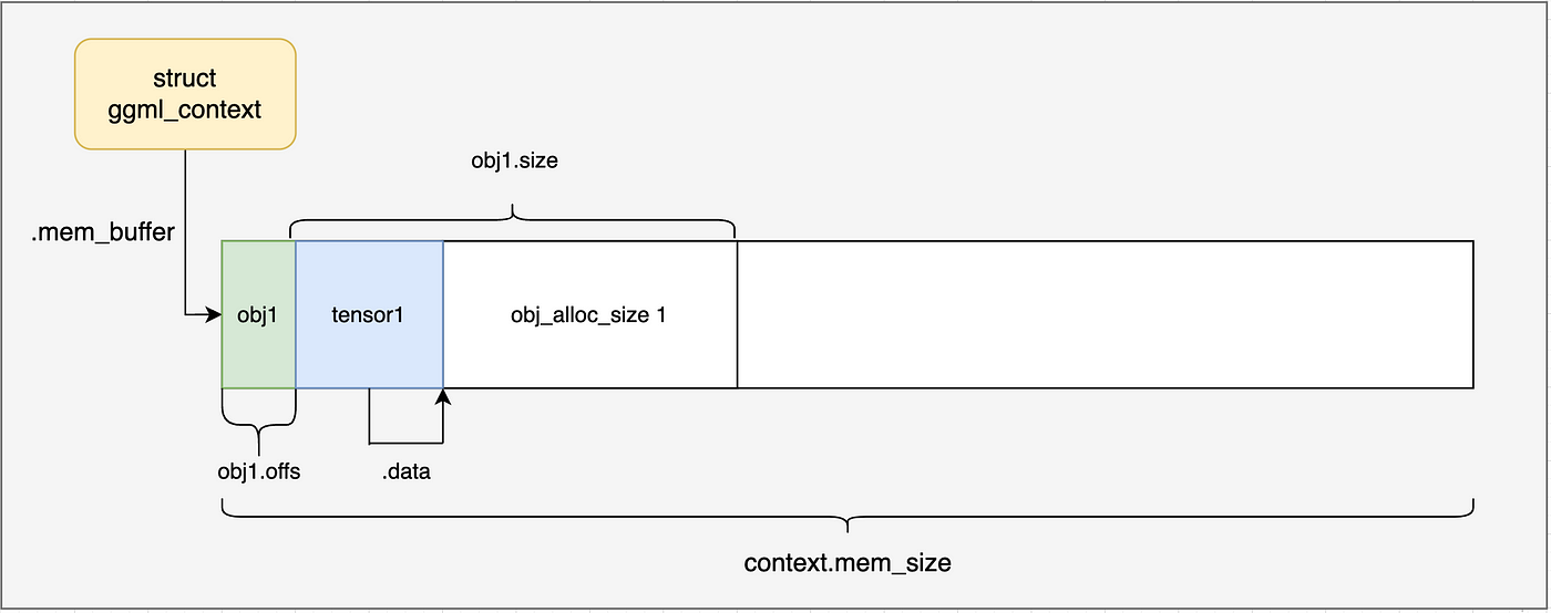
包括了 struct ggml_object的size + struct ggml_tensor的size + obj_alloc_size(也就是tensor的data内存大小)。当然ggml_tensor struc的size和obj_alloc_size还需要进行内存对齐。
到此,我们的ggml_context内存布局(没有分配新的内存,所有的内存都是分配ctx时分配)如下图所示:
ggml_tensor如何定义
上节,我们的第一个tensor,以及通过ggml_object进行了表示管理,并为其在ggml_context中分配了内存,那么ggml_tensor结构体的定义呢?
我们继续看ggml_new_tensor_impl函数中的下半部分内容。
C++ struct ggml_tensor * const result = ( struct ggml_tensor * )(( char * ) ctx -> mem_buffer + obj_new -> offs );
* result = ( struct ggml_tensor ) {
/*.type =*/ type ,
/*.buffer =*/ NULL ,
/*.ne =*/ { 1 , 1 , 1 , 1 },
/*.nb =*/ { 0 , 0 , 0 , 0 },
/*.op =*/ GGML_OP_NONE ,
/*.op_params =*/ { 0 },
/*.flags =*/ 0 ,
/*.src =*/ { NULL },
/*.view_src =*/ view_src ,
/*.view_offs =*/ view_offs ,
/*.data =*/ obj_alloc_size > 0 ? ( void * )( result + 1 ) : data ,
/*.name =*/ { 0 },
/*.extra =*/ NULL ,
/*.padding =*/ { 0 },
};
for ( int i = 0 ; i < n_dims ; i ++ ) {
result -> ne [ i ] = ne [ i ];
}
result -> nb [ 0 ] = ggml_type_size ( type );
result -> nb [ 1 ] = result -> nb [ 0 ] * ( result -> ne [ 0 ] / ggml_blck_size ( type ));
for ( int i = 2 ; i < GGML_MAX_DIMS ; i ++ ) {
result -> nb [ i ] = result -> nb [ i - 1 ] * result -> ne [ i - 1 ];
}
ctx -> n_objects ++ ;
return result ;
result指针指向了ctx->mem_buffer + obj_new->offs,也就是ggml_tensor结构体对象所分配的内存。
ggml_tensor结构体的关键字段如下:
data:指向tensor张量数据存储起始地址,这里就是ggml_tensor结构体自身之后的第一个字节。
ne:一个大小为4的数组,表示每个维度的元素数量,这里是[2, 4, 1, 1]。
nb:一个大小为4的数组,表示每个维度的元素字节数,这里是[4, 8, 32, 32]。
如果不考虑量化,计算方式如下:
C++ nb [ 0 ] = sizeof ( float );
nb [ 1 ] = nb [ 0 ] * ne [ 0 ];
nb [ 2 ] = nb [ 1 ] * ne [ 1 ];
nb [ 3 ] = nb [ 2 ] * ne [ 2 ];
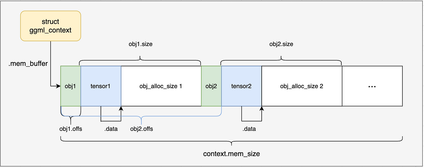
通过上面的内容我们以及了解了ggml_new_tensor_2d的工作原理。在simple-ctx例子中,会调用两次以分配两个tensor张量,一次为x,一次为y,分配后的内存布局如下图所示:
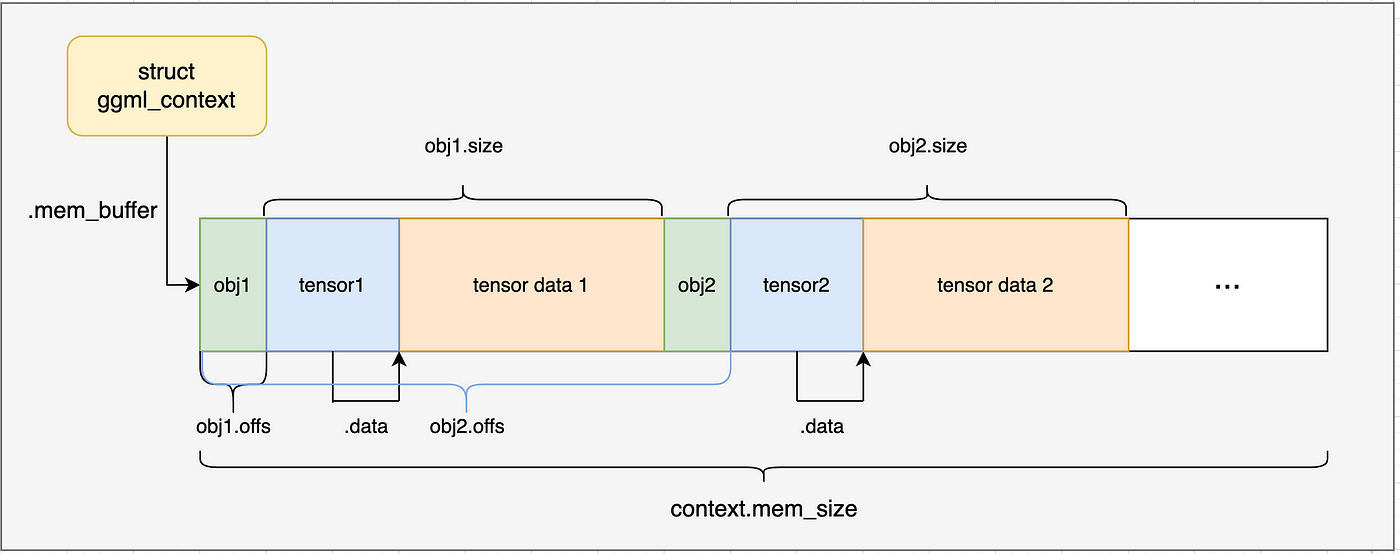
然后通过memcpy将数据复制到ggml_tensor的data字段中。
这里的张量数据直接硬编码定义到了源代码中,因此不需要加载GGU文件,再更复杂的例子中会通过GGU文件加载数据。
要点
ggml 通过ggml_context来处理内存分配
ggml_context中通过链表来管理内存,每个节点都是ggml_object结构体,隐式管理tensor张量、计算图、work buffer等资源。
ggml_tensor的维度表示和pytorch是相反的,这个需要注意。
探索ggml的实现–GGML计算图构建
本小节介绍GGML如何构建和管理计算图相关的数据结构。
在ggml_context中创建计算图
上一节,完成了ggml_context的创建,并且完成了矩阵计算所需的ggml_tensor张量的创建。(load_model函数中实现的功能)
C++ simple_model model ;
load_model ( model , matrix_A , matrix_B , rows_A , cols_A , rows_B , cols_B );
// perform computation in cpu
struct ggml_tensor * result = compute ( model );
接下来重点研究的就是compute函数,分为构建计算图、执行图计算、获取结果(获取最后一个计算节点的输出结果)三个步骤。
C++ // compute with backend
struct ggml_tensor * compute ( const simple_model & model ) {
struct ggml_cgraph * gf = build_graph ( model );
int n_threads = 1 ; // number of threads to perform some operations with multi-threading
ggml_graph_compute_with_ctx ( model . ctx , gf , n_threads );
// in this case, the output tensor is the last one in the graph
return ggml_graph_node ( gf , -1 );
}
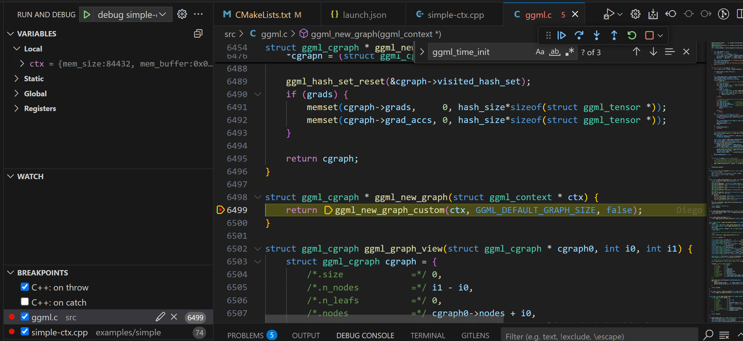
在build_graph函数中,首先会调用ggml_new_graph ,这个函数可以和前一节中ggml_new_tensor函数一样的方式理解。它也是创建了ggml_object对象,但是不同的是,这个object管理的是计算图(ggml_cgraph结构体对象) ,而不是tensor张量。
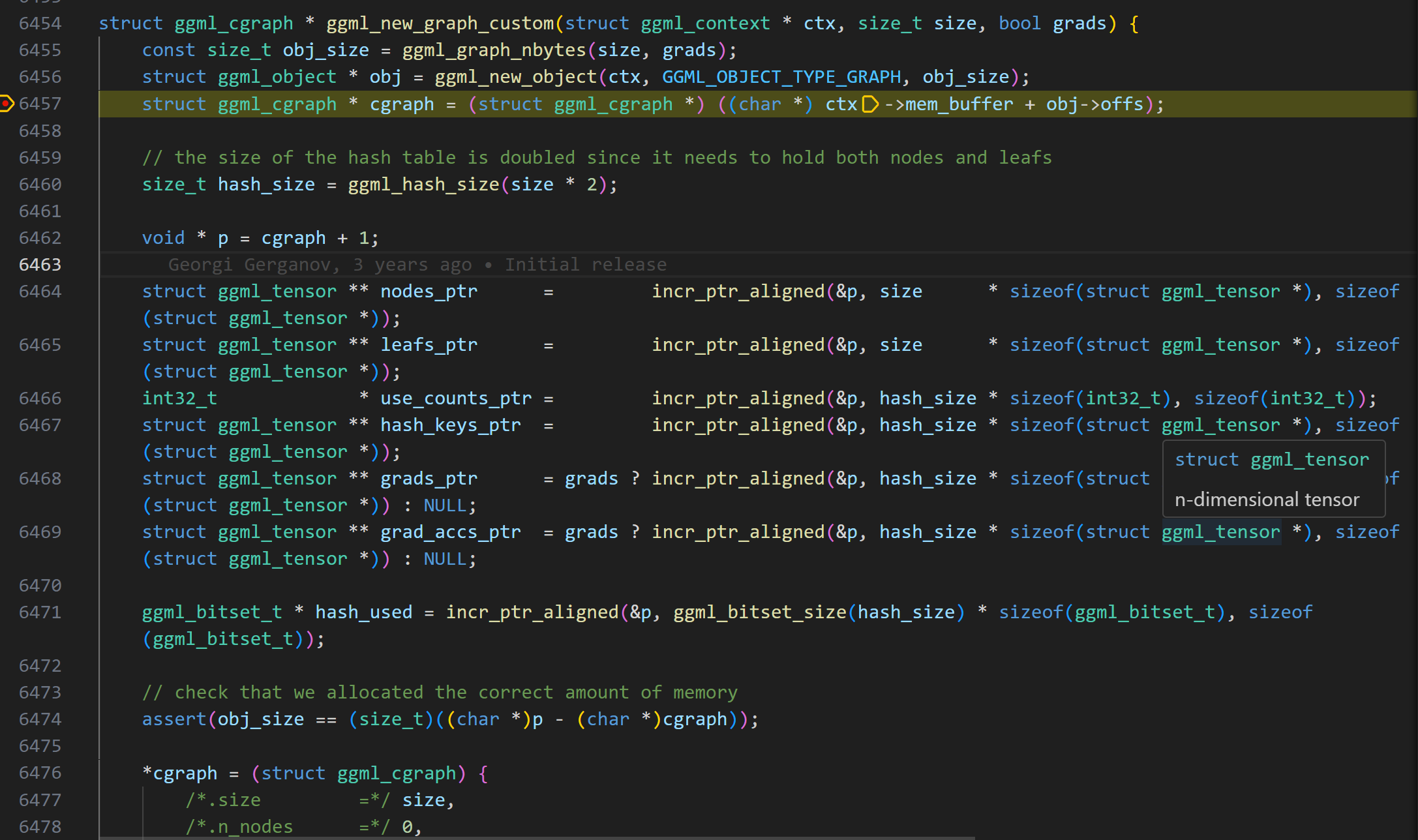
通过ggml_graph_nbytes函数获取计算图需要占用的内存大小
ggml_new_object根据计算图大小在ggml_context内存区域中分配一块内存,创建ggml_object对象
通过offs偏移获取ggml_object中管理的ggml_cgraph结构体对象指针,完成计算图的构建
现在我们再对细节进行展开介绍:
ggml_gral_nbytes计算细节
GGML_DEFAULT_GRAPH_SIZE是一个宏定义,默认值为2048。定义了单个ggml_cgraph中可分配的最大节点树和leaf(叶节点)张量数。然后使用ggml_hash_size函数计算hash表需要的内存大小,乘以2是需要管理nodes和leafs两种类型。
C++ // 调用ggml_new_graph_custom传递的参数
ggml_new_graph_custom ( ctx , GGML_DEFAULT_GRAPH_SIZE , false );
#define GGML_DEFAULT_GRAPH_SIZE 2048
static size_t ggml_graph_nbytes ( size_t size , bool grads ) {
size_t hash_size = ggml_hash_size ( size * 2 );
void * p = 0 ;
incr_ptr_aligned ( & p , sizeof ( struct ggml_cgraph ), 1 );
incr_ptr_aligned ( & p , size * sizeof ( struct ggml_tensor * ), sizeof ( struct ggml_tensor * )); // nodes
incr_ptr_aligned ( & p , size * sizeof ( struct ggml_tensor * ), sizeof ( struct ggml_tensor * )); // leafs
incr_ptr_aligned ( & p , hash_size * sizeof ( int32_t ), sizeof ( int32_t )); // use_counts
incr_ptr_aligned ( & p , hash_size * sizeof ( struct ggml_tensor * ), sizeof ( struct ggml_tensor * )); // hash keys
if ( grads ) {
incr_ptr_aligned ( & p , hash_size * sizeof ( struct ggml_tensor * ), sizeof ( struct ggml_tensor * )); // grads
incr_ptr_aligned ( & p , hash_size * sizeof ( struct ggml_tensor * ), sizeof ( struct ggml_tensor * )); // grad_accs
}
// 计算hash_size需要多少个ggml_bitset_t表示状态,这些多个ggml_bitset_t构成了bit位图
incr_ptr_aligned ( & p , ggml_bitset_size ( hash_size ) * sizeof ( ggml_bitset_t ), sizeof ( ggml_bitset_t ));
size_t nbytes = ( size_t ) p ;
return nbytes ;
}
ggml_hash_size从其实现来看,通过二分查找找到大于或等于2 * GGML_DEFAULT_GRAPH_SIZE的最小质数,这个质数决定了计算图哈希表的大小。选择质数主要是出于性能考虑:GGML采用了一种简单的开放地址哈希函数,并使用线性探测法。
C++ // the last 4 bits are always zero due to alignment
Key = ( ggml_tensor_pointer_value >> 4 ) % table_size
使用质数表大小有助于更均匀地分布键,减少聚集、提高查找效率。
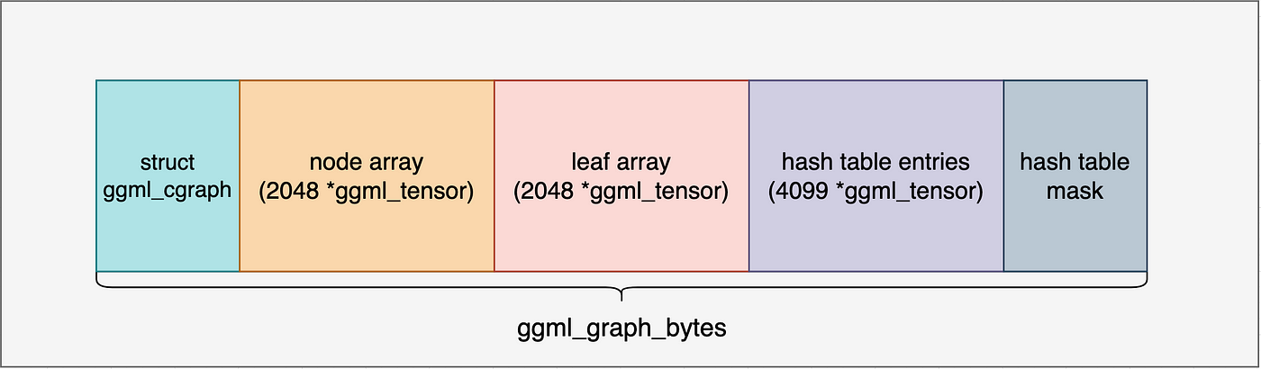
ggml_graph的内存布局:
ggml_cgraph结构体对象占用空间:sizeof(struct ggml_cgraph)
2048个tensor张量指针,指向nodes
2048个tensor张量指针,指向leafs
hash_size个int32_t,用于记录张量的使用次数
hash_size个tensor张量指针,用于存储张量的哈希键
梯度相关,simple_ctx例子不涉及
哈希表bit位图,用于记录张量的使用情况
关于bit位图,
C++ typedef uint32_t ggml_bitset_t ;
static_assert ( sizeof ( ggml_bitset_t ) == 4 , "bitset_t constants must be updated" );
#define BITSET_SHR 5 // log2(sizeof(ggml_bitset_t)*8)
#define BITSET_MASK (sizeof(ggml_bitset_t)*8 - 1)
// >> BITSET_SHR相当于除以32,表示数字n的bit记录位于第几个ggml_bitset_t中
// 一个ggml_bitset_t可以表示32个数的状态,在本文上下文中即表示一个hash位置
static size_t ggml_bitset_size ( size_t n ) {
return ( n + BITSET_MASK ) >> BITSET_SHR ;
}
根据ggml_graph_nbytes函数计算出来的内存大小,在ctx中分配内存,分配后的内存布局如下:
包括计算图对象、节点指针、叶子指针、使用次数、哈希键、梯度、哈希表bit位图。接下来的几行代码初始化指向已分配内存中不同区域的指针,并将它们存储在ggml_cgraph结构体中。最后,哈希表被重置,所有槽位都被标记为未占用。
构建矩阵乘计算图
前面的内容介绍了在ggml_context中分配一个计算图内存,并且初始化了相关成员默认值。
C++ struct ggml_cgraph * gf = ggml_new_graph ( model . ctx );
// 用gf表示矩阵乘任务
// result = a*b^T
struct ggml_tensor * result = ggml_mul_mat ( model . ctx , model . a , model . b );
ggml_build_forward_expand ( gf , result );
现在这个计算图gf支持添加2048个张量节点和叶节点,但是还没有将矩阵乘这个计算的节点加入计算图。接下来的内容就是介绍如何将矩阵乘任务信息用计算图进行表示。
在ggml_mul_mat函数中,首先检查输入张量的合法性,然后创建一个结果张量,并设置张量的运算类型为矩阵乘。
C++ struct ggml_tensor * ggml_mul_mat (
struct ggml_context * ctx ,
struct ggml_tensor * a ,
struct ggml_tensor * b ) {
GGML_ASSERT ( ggml_can_mul_mat ( a , b ));
GGML_ASSERT ( ! ggml_is_transposed ( a ));
// 计算结果的shape
const int64_t ne [ 4 ] = { a -> ne [ 1 ], b -> ne [ 1 ], b -> ne [ 2 ], b -> ne [ 3 ] };
struct ggml_tensor * result = ggml_new_tensor ( ctx , GGML_TYPE_F32 , 4 , ne );
// 将加入graph nodes中的一个node,类型位矩阵乘
result -> op = GGML_OP_MUL_MAT ;
result -> src [ 0 ] = a ;
result -> src [ 1 ] = b ;
return result ;
}
现在,到了我们构建计算图的最后阶段了,秘密就藏在ggml_build_forward_expand函数中。
函数的输入参数是我们创建的“空图”和矩阵乘任务所返回的矩阵乘结果节点(在复杂的案例中,就是模型的输出节点或者LLM中的logits)。
ggml_build_forward_expand 函数细节探索
该函数调用到了ggml_build_forward_impl函数,核心实现在ggml_visit_parents中。
C++ static void ggml_build_forward_impl ( struct ggml_cgraph * cgraph , struct ggml_tensor * tensor , bool expand ) {
const int n0 = cgraph -> n_nodes ;
ggml_visit_parents ( cgraph , tensor );
const int n_new = cgraph -> n_nodes - n0 ;
GGML_PRINT_DEBUG ( "%s: visited %d new nodes \n " , __func__ , n_new );
if ( n_new > 0 ) {
// the last added node should always be starting point
GGML_ASSERT ( cgraph -> nodes [ cgraph -> n_nodes - 1 ] == tensor );
}
}
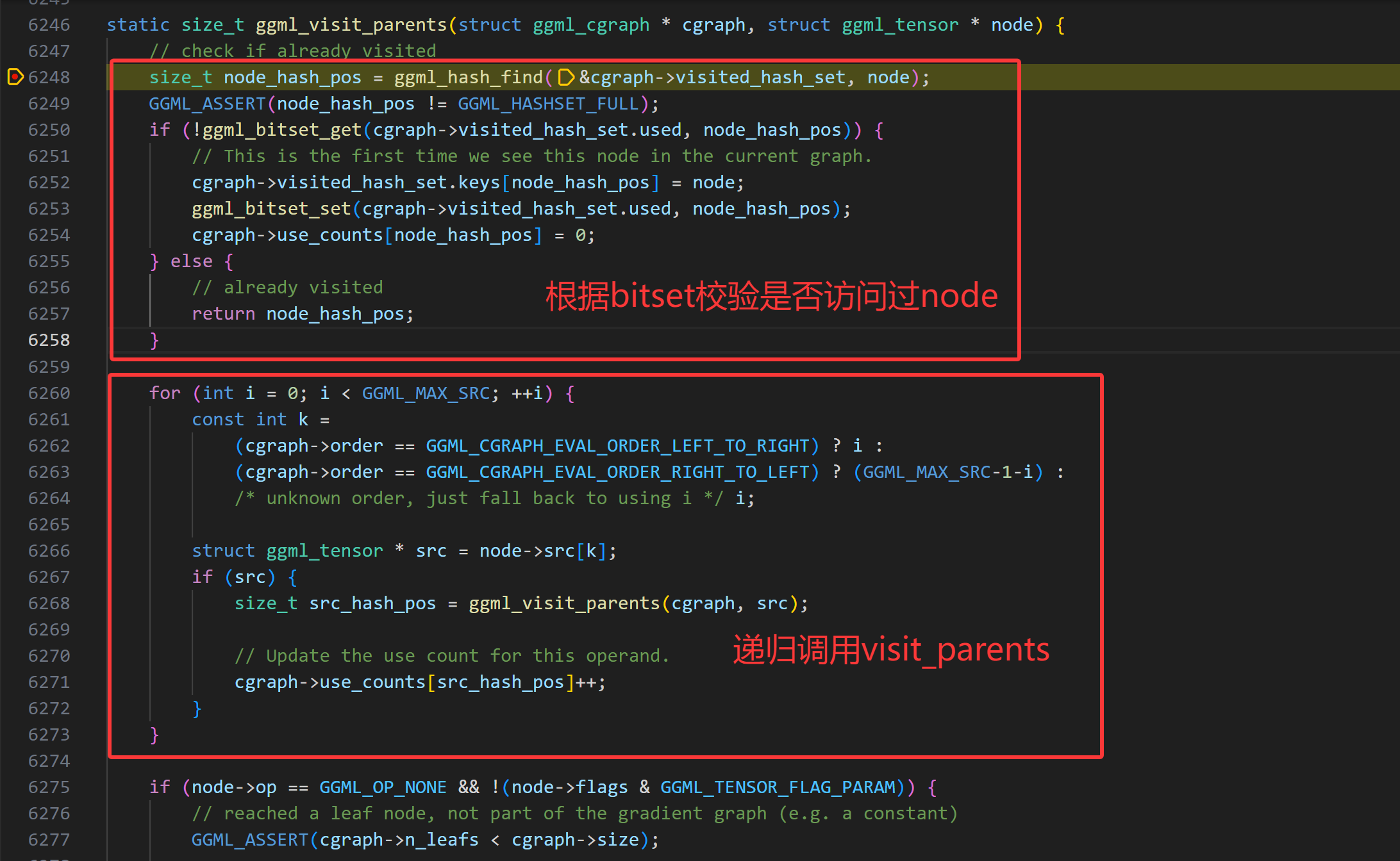
ggml_visit_parents函数通过递归的方式构建了计算图。
核心逻辑:
检查当前张量是否已存在于哈希表中。如果存在,则停止执行并返回。
对所有src张量递归调用ggml_visit_parents函数。
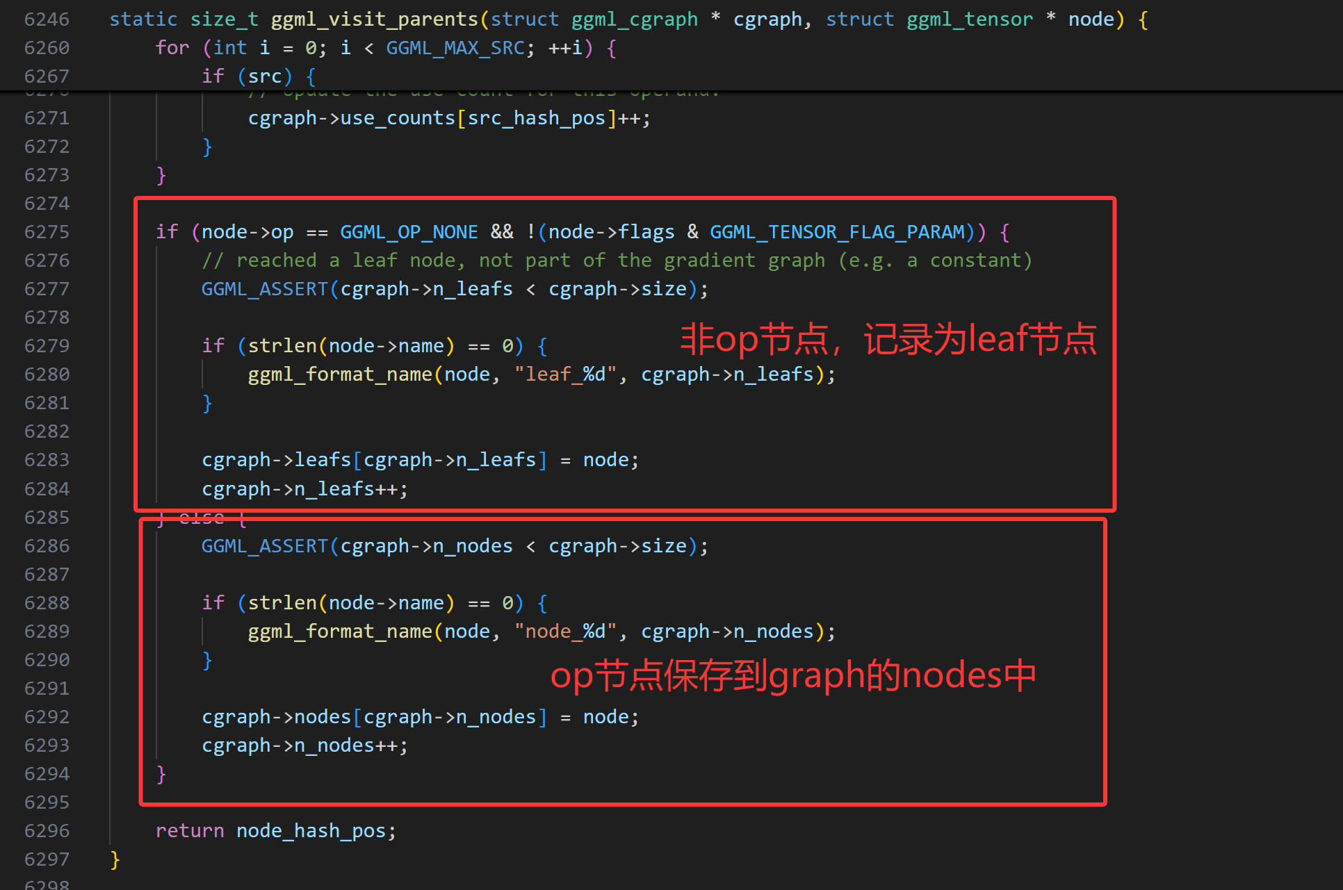
如果它是一个叶节点(即常量张量或不由运算生成的输入张量),则将其存储在图的叶数组(leafs数组)中。
否则,将其存储在图的节点数组(nodes数组)中。
所有递归调用返回后,最后一次检查会确保最后记录的节点是结果张量。因为使用了后序遍历,这意味着输入节点(张量)是最后插入的。
采用debug打印gf计算图信息,1个node节点就是mat mul op节点,两个leaf节点就是两个输入张量a、b矩阵。
C++ > p * gf
( ggml_cgraph ) {
size = 2048
n_nodes = 1
n_leafs = 2
nodes = 0x000055555556ddd8
grads = nullptr
grad_accs = nullptr
leafs = 0x0000555555571dd8
use_counts = 0x0000555555575dd8
visited_hash_set = {
size = 4099
used = 0x0000555555581e00
keys = 0x0000555555579de8
}
order = GGML_CGRAPH_EVAL_ORDER_LEFT_TO_RIGHT
}
到目前为止,我们已经构建好了a、b矩阵乘这个任务的计算图,接下来就是看GGML如何执行这个计算图并获取计算结果了。
探索ggml的实现–执行GGML计算图
这节主要介绍如何计算GGML计算图,实现的核心逻辑在ggml_graph_compute_with_ctx函数中。
C++ int n_threads = 1 ; // number of threads to perform some operations with multi-threading
ggml_graph_compute_with_ctx ( model . ctx , gf , n_threads );
// in this case, the output tensor is the last one in the graph
return ggml_graph_node ( gf , -1 );
在该函数中,首先创建了个一个计算计划,并且根据cplan的work_size分配了完成这个plan所需的buffer,然后调用ggml_graph_compute函数执行计算计划。
C++ enum ggml_status ggml_graph_compute_with_ctx ( struct ggml_context * ctx , struct ggml_cgraph * cgraph , int n_threads ) {
struct ggml_cplan cplan = ggml_graph_plan ( cgraph , n_threads , NULL );
cplan . work_data = ( uint8_t * ) ggml_new_buffer ( ctx , cplan . work_size );
return ggml_graph_compute ( cgraph , & cplan );
}
ggml_cplan结构体的核心目的是:确定计算的关键执行参数 。
探索ggml_graph_plan细节
如何确定线程数量
ggml_graph_plan函数实现的主要功能就是确定计算计划所需的线程数和临时内存大小。
确定线程数的逻辑:
C++ final_n_threads = MIN ( n_threads , MAX ( each node ' s maximum multithreading count ))
确定工作缓存区大小
在simple-ctx这个例子中,threads_count = 1, work_buffer_size = 0。在接下来的函数ggml_new_buffer中,可以看到分配的work_buffer_size大小的缓存区,也是在context的内存buffer中分配的。
C++ > p cplan
( ggml_cplan ) {
work_size = 0
work_data = 0x00005555555821d0 ""
n_threads = 1
threadpool = NULL
abort_callback = 0x0000000000000000
abort_callback_data = 0x0000000000000000
}
计算图的执行计算
到目前为止,为了执行计算图,已经准备好了张量数据、计算图、计算计划(plan),执行的关键逻辑来到了ggml_graph_compute函数,将计算图cgraph和cplan作为参数传入。
C++ ggml_graph_compute ( cgraph , & cplan );
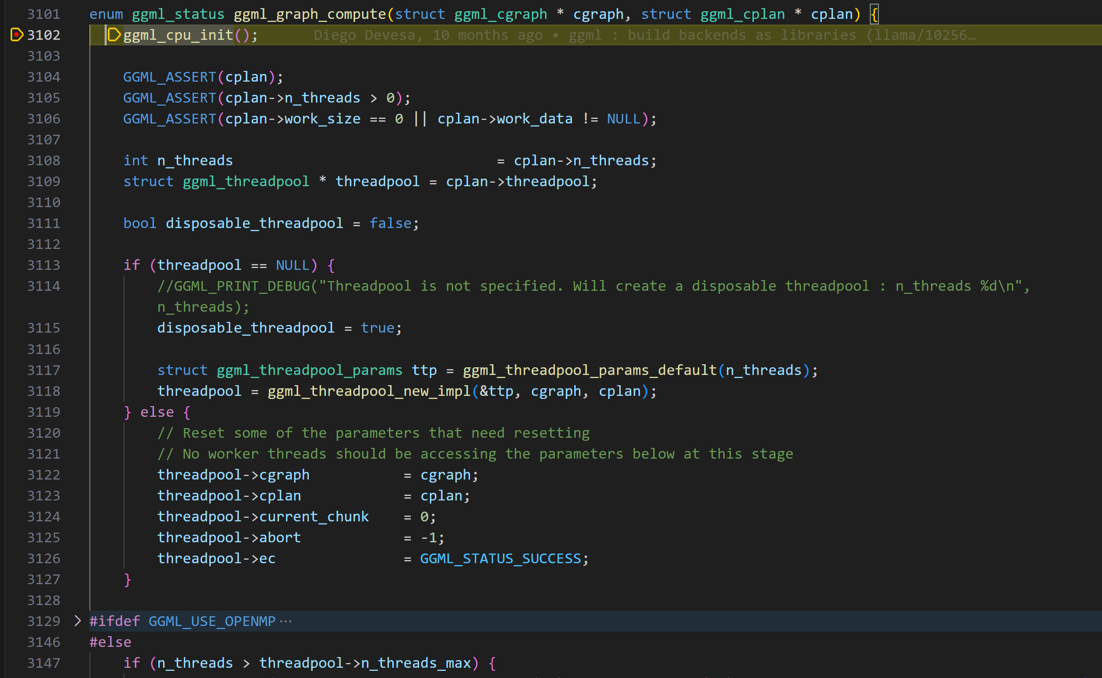
在ggml_graph_compute函数中, 实现了如下核心功能:
在ggml_cpu_init函数中,创建了一些快速计算的查找表。比如f32到f16的转换表、gelu计算的查找表。
C++ ggml_table_f32_f16 [ i ] = f ;
ggml_table_gelu_f16 [ i ] = GGML_CPU_FP32_TO_FP16 ( ggml_gelu_f32 ( f ));
ggml_table_gelu_quick_f16 [ i ] = GGML_CPU_FP32_TO_FP16 ( ggml_gelu_quick_f32 ( f ));
创建了线程池,将计算图和计算任务dispath给线程池执行。在linux下,ggml采用pthread实现线程相关操作。(关于GGML_USE_OPENMP的逻辑可以先跳过)
GGML线程池实现
GGML 实现了一个线程池,该线程池经过优化,可高效运行计算图,并针对 NUMA 架构进行了优化。
ggml首先使用默认参数初始化一个ggml_thread_pool结构体,然后为每个工作线程分配一个状态结构体(ggml_compute_state),负责线程池中的每个线程的状态记录:
C++ // Per-thread state
struct ggml_compute_state {
#ifndef GGML_USE_OPENMP
// linux下实际为pthread
ggml_thread_t thrd ;
// 用于设置cpu亲和性(NUMA相关优化)
bool cpumask [ GGML_MAX_N_THREADS ];
int last_graph ;
bool pending ;
#endif
// 指向线程池的指针
struct ggml_threadpool * threadpool ;
// 线程编号
int ith ;
};
如果启用了 OpenMP,线程管理会自动处理;否则,GGML 会手动创建和管理 pthread,即手动设置cpu亲和性等操作。
cpu亲和性设置
由于在numa架构下,本地/远程内存访问速度差异大,通过NUMA感知调度(如线程绑定、内存分配优化)可提升性能。通过设置cpu亲和性,绑定线程到本地NUMA节点,减少远程访问。
在ggml的实现中,通过函数ggml_thread_cpumask_next()为每个worker线程分配cpu亲和性。
C++ static void ggml_thread_cpumask_next ( const bool * global_mask , bool * local_mask , bool strict , int32_t * iter ) {
if ( ! strict ) {
memcpy ( local_mask , global_mask , GGML_MAX_N_THREADS );
return ;
} else {
memset ( local_mask , 0 , GGML_MAX_N_THREADS );
int32_t base_idx = * iter ;
for ( int32_t i = 0 ; i < GGML_MAX_N_THREADS ; i ++ ) {
int32_t idx = base_idx + i ;
if ( idx >= GGML_MAX_N_THREADS ) {
// Just a cheaper modulo
idx -= GGML_MAX_N_THREADS ;
}
if ( global_mask [ idx ]) {
local_mask [ idx ] = 1 ;
* iter = idx + 1 ;
return ;
}
}
}
}
在该函数中通过strict参数控制线程的亲和性设置。
这种逻辑确保线程在可用的CPU核心之间均匀分布,从而减少竞争。
计算图工作线程创建及调度
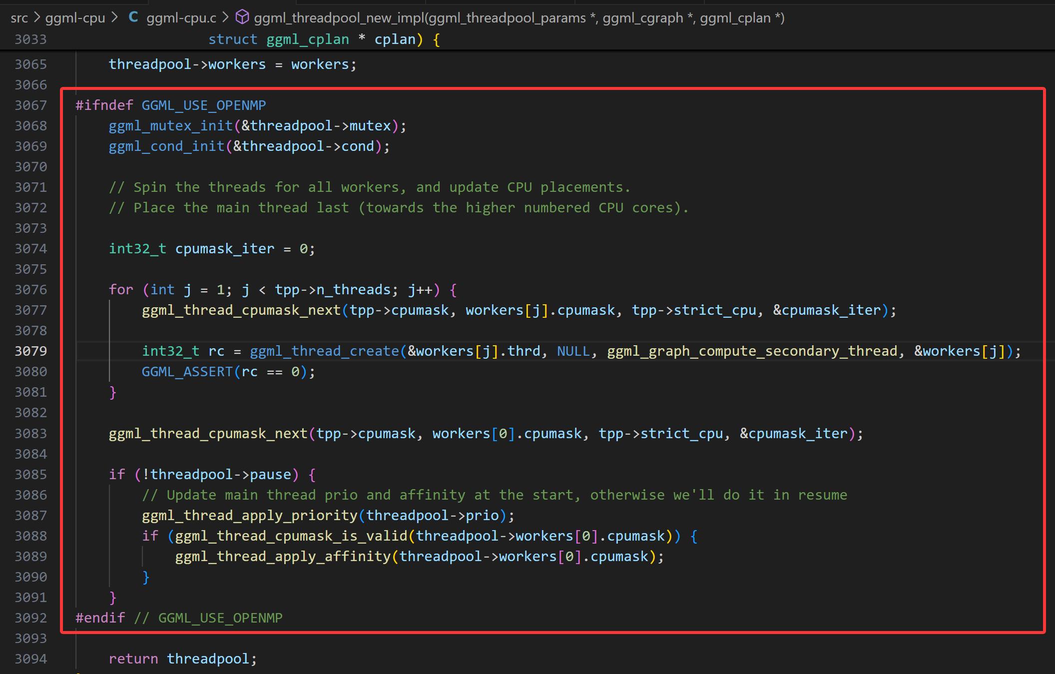
上面的逻辑完成了线程池的创建、亲和性的设置,接下来就是创建具体的工作线程了,也就是线程跑起来要执行怎样的运算逻辑。
注意,这里创建工作线程是从thread 1开始的,因为thread 0的触发不在这里。
C++ for ( int j = 1 ; j < tpp -> n_threads ; j ++ ) {
int32_t rc = ggml_thread_create ( & workers [ j ]. thrd , NULL , ggml_graph_compute_secondary_thread , & workers [ j ]);
}
接下来,请看ggml_graph_compute_secondary_thread函数。
C++ static thread_ret_t ggml_graph_compute_secondary_thread ( void * data ) {
struct ggml_compute_state * state = ( struct ggml_compute_state * ) data ;
struct ggml_threadpool * threadpool = state -> threadpool ;
// 设置线程优先级
ggml_thread_apply_priority ( threadpool -> prio );
if ( ggml_thread_cpumask_is_valid ( state -> cpumask )) {
// 设置线程 affinity
ggml_thread_apply_affinity ( state -> cpumask );
}
while ( true ) {
// Check if we need to sleep
while ( threadpool -> pause ) {
GGML_PRINT_DEBUG ( "thread #%d inside pause loop \n " , state -> ith );
ggml_mutex_lock_shared ( & threadpool -> mutex );
if ( threadpool -> pause ) {
ggml_cond_wait ( & threadpool -> cond , & threadpool -> mutex );
}
GGML_PRINT_DEBUG ( "thread #%d resuming after wait \n " , state -> ith );
ggml_mutex_unlock_shared ( & threadpool -> mutex );
}
// This needs to be checked for after the cond_wait
if ( threadpool -> stop ) break ;
// Check if there is new work
// The main thread is the only one that can dispatch new work
ggml_graph_compute_check_for_work ( state );
if ( state -> pending ) {
state -> pending = false ;
ggml_graph_compute_thread ( state );
}
}
return ( thread_ret_t ) 0 ;
}
让我们回头看看主线程中的ggml_graph_compute逻辑,它首先创建线程池,也就是上面的部分。创建好从1开始的工作线程后,然后调用了ggml_graph_compute_kickoff,就是它把线程池的pause设置为false。
然后线程0在这个启动其它线程的线程开始执行ggml_graph_compute_thread计算任务。
C++ enum ggml_status ggml_graph_compute ( struct ggml_cgraph * cgraph , struct ggml_cplan * cplan ) {
// Kick all threads to start the new graph
ggml_graph_compute_kickoff ( threadpool , n_threads );
// This is a work thread too
ggml_graph_compute_thread ( & threadpool -> workers [ 0 ]);
}
多线程如何执行矩阵乘张量计算
GGML的所有线程每次只处理一个节点。让我们看看ggml_compute_forward,其中会根据节点的运算符类型选择实际的计算函数。这是通过一个庞大的switch-case语句块来处理的。
C++ static thread_ret_t ggml_graph_compute_thread ( void * data ) {
struct ggml_compute_state * state = ( struct ggml_compute_state * ) data ;
struct ggml_threadpool * tp = state -> threadpool ;
const struct ggml_cgraph * cgraph = tp -> cgraph ;
const struct ggml_cplan * cplan = tp -> cplan ;
set_numa_thread_affinity ( state -> ith );
struct ggml_compute_params params = {
/*.ith =*/ state -> ith ,
/*.nth =*/ atomic_load_explicit ( & tp -> n_threads_cur , memory_order_relaxed ),
/*.wsize =*/ cplan -> work_size ,
/*.wdata =*/ cplan -> work_data ,
/*.threadpool=*/ tp ,
};
for ( int node_n = 0 ; node_n < cgraph -> n_nodes && atomic_load_explicit ( & tp -> abort , memory_order_relaxed ) != node_n ; node_n ++ ) {
struct ggml_tensor * node = cgraph -> nodes [ node_n ];
ggml_compute_forward ( & params , node );
if ( state -> ith == 0 && cplan -> abort_callback &&
cplan -> abort_callback ( cplan -> abort_callback_data )) {
atomic_store_explicit ( & tp -> abort , node_n + 1 , memory_order_relaxed );
tp -> ec = GGML_STATUS_ABORTED ;
}
if ( node_n + 1 < cgraph -> n_nodes ) {
ggml_barrier ( state -> threadpool );
}
}
ggml_barrier ( state -> threadpool );
return 0 ;
}
C++ case GGML_OP_MUL_MAT :
{
ggml_compute_forward_mul_mat ( params , tensor );
} break ;
查看ggml_compute_forward_mul_mat的实现可知,矩阵的计算不是一个线程完成整个矩阵的计算,而是传递了thread_id参数,根据thread_id来拆分矩阵块,分块计算。
这里也可以看到GGML的计算图执行调度和一般图计算的区别,一般场景的有向无环图,多个线程并行执行多个可以并行的node,这里GGML是一次只执行一个node,node中多个线程分块计算。然后进入下一个节点计算。
一旦一个节点node的计算完成,所有线程都会在屏障ggml_barrier处同步,确保它们在进入下一个节点之前完成当前节点的计算。这个过程会重复进行,直到图中的所有节点都被评估完毕。
上面更多的谈到的是不使用OpenMP,手动管理线程的凡是。如果启用OpenMP后,它会自动管理并行计算,无需手动创建和同步线程。我们无需自己处理线程池、条件变量和竞争条件,只需设置线程数量,让每个线程执行ggml_graph_compute_thread即可。
获取计算结果
C++ // perform computation in cpu
struct ggml_tensor * result = compute ( model );
// get the result data pointer as a float array to print
std :: vector < float > out_data ( ggml_nelements ( result ));
memcpy ( out_data . data (), result -> data , ggml_nbytes ( result ));
// expected result:
// [ 60.00 55.00 50.00 110.00
// 90.00 54.00 54.00 126.00
// 42.00 29.00 28.00 64.00 ]
最后就是获取result node,然后将计算结果拷贝出来。到此,通过simple-ctx的例子,我们从源码理解了GGML如何实现在ggml_context中分配所有需要的内存,通过cpu backend的方式执行计算图。